


Quantum Computing is at an experimental stage but is already showing potential to impact many organizations and their current business solutions. What steps can an organization take to be prepared for the coming era of Quantum Computing, and what must they be wary of? A use case around portfolio optimization is presented to help the reader conceptualize how a business problem can be solved using Quantum Computing.
Introduction
Quantum Computing is continuing its climb out of the depths of laboratories and is gaining more and more traction in the business world ([McKi21]). In our previous Compact article [Goen21], we gave an introduction to Quantum Computing. In this article, we will get hands-on and show what steps an organization can take to become quantum-ready.
Our digital economy relies strongly on our trust in cybersecurity: cryptographic algorithms ensure that our data can only be used by those who should have access to it. Quantum computers might render some of these algorithms unsafe by leveraging their unique processing power to intercept and decrypt messages. Having a better understanding of the possibilities of Quantum Computing will help identify future cybersecurity threats ([Lipm21]). While these threats should definitely not be overlooked, we will focus in this article on all the benefits that Quantum Computing brings.
Quantum computers run algorithms in such a different manner that they have the potential to outperform the algorithms your organization currently employs by several orders of magnitude. Understanding how quantum computers achieve this might seem like a daunting task at first, but it doesn’t have to be. Just like a programmer does not need to know how the CPU in your computer processes binary signals, developing quantum software doesn’t require a full understanding of quantum physics. We can distinguish between different levels of expertise needed at various stages of the development of a quantum-computing based data analysis.
Quantum Computing is currently said to be in the noisy intermediate-scale quantum (NISQ) era, which means that the leading quantum processors contain up to a few hundred quantum bits (qubits), but these are not advanced enough to reach fault-tolerance nor large enough to really profit from quantum supremacy. It may well take up to 5 or 10 years before Quantum Computing will be integrated into everyday life ([Marr21]). Meanwhile, developments of simulated quantum hardware are already showing promising results in areas of general optimization, simulation processes, machine learning, and cryptographic processes ([Dilm22]). When Quantum Computing becomes available at full scale, its impact will be even larger. Being quantum-ready as an organization means being prepared for the potential benefits but also for the threats that the arrival of Quantum Computing brings, and can be divided in five steps ([Prot21], [Carr21]).
The five steps an organization can take to become quantum-ready
The five steps illustrated in Figure 1 outline what an organization can undertake to become quantum-ready. The steps are explained in further detail down below.
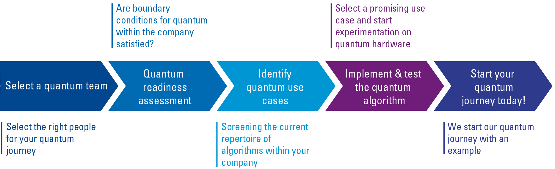
Figure 1. Five steps an organization can take to become quantum-ready. [Click on the image for a larger image]
Step 1: Select a quantum team
Your quantum journey starts by selecting a quantum champion. This quantum champion manages the learning trajectory ([Yndu19]) and should be a generalist in the field of Quantum Computing and a good communicator. The quantum champion is also the one in charge of the quantum readiness assessment of Step 2. Alongside the quantum champion, a data scientist or engineer, with a background in mathematics or computer science for example, oversees the models and algorithms currently driving your organization. Their main concern will be to determine the complexity of these models and algorithms, and select use-cases that could benefit from Quantum Computing. In Step 3. finally, a software engineer can aid in the implementation of the actual algorithm, that will be described in Step 4. And naturally, your team will grow over time as the advantages of Quantum Computing become more and more visible!
Step 2: Quantum readiness assessment
Next, the quantum champion should assess whether or not the boundary conditions are satisfied to carry out a Quantum Computing-based analysis within the company. Is there willingness to adapt changes? Do the current team members have the skills required to successfully carry out a quantum-based analysis? Is budget available to perform research and development (R&D)? And lastly, are there potential partners in R&D and technology, both internal and external, that can support the work to be done?
Step 3: Identify Quantum Computing use cases
While quantum computers cannot solve any problems that classical computers cannot already solve, quantum computers might solve certain problems faster than classical computers. Identifying use cases starts by screening the current repertoire of algorithms that is being deployed within your organization. Assessing the complexity of these algorithms might help to choose between classic or quantum-based optimization approaches.
Computers can be used to solve problems by translating these problems into a mathematical model, which in turn is implemented as an algorithm: a sequence of well-defined steps, that either provide an exact or approximate solution to your problem. The number of steps an algorithm requires to obtain the solution defines the complexity of the problem. We do not exactly count those steps, but describe complexity as a function of the number of variables of the problem. To illustrate this, consider that we want to find a specific book in an enourmous pile of n books. If its happens to be the first book you check, you’re in luck. But in the worst case, it might require checking all book. Because you have to check each book once, we say this problem linear complexity, which we write as O(n). If we add or remove one book to the pile, only the additional book needs to be checked if you want to know if the new pile contains your book. But now consider that we want to sort the pile of books. Simple sorting of a set of books has quadratic complexity, written as O(n2) , as adding one book to the pile requires us to check first where we must insert it, which by itself aleady takes additional steps (although there are slightly smarter ways to do so). The so-called Big notation expresses how the run-time of an algorithm is related to the input size of the problem. Whenever the complexity function is a polynomial function of n, such as n2 or maybe n14, the problem would be classified as a polynomial-time problem.
Quantum Computing might help solving problems by reducing their complexity, meaning that fewer steps are required to solve the problem on a quantum computer by exploiting properties of quantum mechanics. An example of this is Grover’s algorithm for finding an item in a set, with a complexity of O(n) on classical computers, as we saw above. But in its quantum form, it has a complexity of O(√n), meaning a quadratic decrease of complexity ([Nikh21]). Part of quantum-readiness entails knowing which types of problems have a quantum implementation with reduced complexity with respect to their classical implementations. Assessing the complexity of an algorithm is specialistic work which requires knowledge of mathematics and computer science, but does not require knowledge of Quantum Computing. Part of becoming quantum-ready could comprise literature study to find out if the complexity of commonly faced analyses within your company are known, and if Quantum Computing could be a relevant alternative for those problems.
Another occasion in which Quantum Computing can outperform classical methods is in heuristic problem solving. Heuristics are algorithms that aim to quickly obtain a reasonably good solution to the problem at hand. Computing the exact solution might be impossible or too time-consuming, while a near-optimal solutions is almost always sufficient in practice. In heuristic problem solving, computational complexity is still of importance, but even more so is the quality of the obtained solution. Quantum heuristics could provide an alternative to classical heuristics by being able to obtain a higher-quality solution with the same run time.
Step 4: Implement the quantum algorithm and put it to the test
A lower complexity is a very strong indication that the quantum algorithm will outperform a classical algorithm when the number of variables is large enough (which can be hundreds or thousands or more, depending on the problem you take), but the overhead of putting the problem in the right format, or migrating data so that it is accessible by the quantum computer, might be substantial.
The true benefit of Quantum Computing becomes really clear when tested in an experimental setting. With experimentation, differences in performance between the quantum-based solution and the classical solution can be quantified. Performance can be measured in various terms, such as speed, resource usage, but also the accuracy of the found solution in case of a heuristic method that obtains an approximate solution.
The good news is that you don’t have to buy a quantum computer to perform experiments on it. Cloud-based quantum computers are available within a few clicks for experimentation. To lower the barrier of implementing quantum algorithms, cloud providers such as IBM and Microsoft host software that helps to translate the logical steps in an algorithm to “quantum building blocks” ([QCR21], [Micr22a]). Performing experiments on actual quantum hardware helps you to understand certain nuances of Quantum Computing, such as its noise and the probabilistic nature of these systems. However, the small number of qubits currently available in these systems does not allow for experimentation with full-scale problems. Alternatively, quantum simulators can be used. Simulators, such as IBM’s QASM Simulator or Microsofts QDK full state simulator ([Micr22b]), provide the opportunity to gather hands-on experience without using costly quantum hardware. While simulating quantum algorithms on classical hardware can be orders of magnitudes slower than simply solving the problem with a classical algorithm, it does allow you to get experience with the underlying mechanics, and porting the problem to real quantum computers will be straightforward.
Step 5: Start the quantum journey!
As an example, we start our quantum journey with a quantum-based portfolio optimization, the steps of which are explained below. Note that we aim to help you, as a reader, to understand the process of developing a quantum-based analysis. Technical details not needed for understanding this process are omitted to keep this section somewhat brief.
Use case: portfolio optimization
Let’s take a look at an example of a bank that likes to ensure that the shares and bonds that it holds in its portfolio provide a desired balance between being profitable while limiting risk. Markowitz (1952) developed a model, which looks at maximizing return by accepting a quantifiable amount of risk ([Mark52]). We define the expected return of the portfolio as E(R)p = ∑iaiE(R)i, where Ri is the return on asset i and ai is the amount of the asset in the portfolio. The risk of the portfolio is quantified by its variance, given by Var(R) = ∑i ∑jaiajCov(Ri, Rj) is the variance of Rp where ai and aj are different assets and Cov(Ri, Rj) are the covariance of the periodic returns of the two assets. The variance describes the volatility of the value of the assets. Markowitz states that the optimal portfolio maximizes profit, and minimizes volatility. The objective for finding the optimal portfolio can therefore be expressed as:
min(–E(R) + Var(R))
Using matrix formulation, this can be written as summations of linear equations:
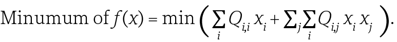
Where Q is a matrix with components and xi ∊ {0, 1}, where 0 means an asset is excluded from the portfolio, and 1 denotes inclusion. This can then be written as:
Min(cx + xQx) with x ∈{0,1},
by replacing the explicit summations with scalar products over vectors c, x, and matrix Q.
QUBO problem formulation and the Ising model
The problem formulated above belongs to the class that is commonly referred to as Quadratic Unconstrained Binary Optimization (QUBO) problems. Many combinatorial problems can be expressed as a QUBO problem. The problem is quadratic, as this is the highest polynomial order of variable x. As all the boundary conditions are enclosed in matrix Q, the problem is unconstrained. Lastly, the problem is binary because x can only assume the values 0 or 1. QUBO problems fall into the NP-hard (non-deterministic polynomial time) complexity class, and may be a good candidate for quantum-based solutions. Interestingly, QUBO’s have an extensively studied analogue in physics: the Ising model. The Ising model was initially developed as a simplified mathematical model to describe the ferromagnetic properties of a material consisting of atoms in a lattice structure. These atoms have a particular property, their dipole moment, which can assume discrete values of –1 or 1. The sum over all dipole moments explains if a material is magnetic or not: if most moments have the same value (either –1 or 1), the sum is large, and the material magnetic. If the moments have random values, they will cancel each other out, and the material is not magnetic.
It may be difficult to see the usefulness of the Ising model in the context of a QUBO at first glance, so let’s look at the details. In the Ising model, the dipole moments of each atom can be affected in two ways: the dipole moment of their neighboring atoms, and a magnetic field acting as external force. The external force may try to align all moments into a particular direction, say +1. Neighboring atoms, however, might prefer to anti-align their magnetic moments, and work against this alignment. Because of this, an Ising model will tend to an equilibrium configuration. The total energy of a system is often expressed in forms of the Hamiltonian H, which for an Ising model of i atoms and <i,j> neighboring pairs, is given by:
H = ∑i∑jJi,jsisj + ∑ihisi
In this expression, the first notation describes the interactions between neighboring atoms, where si and sj are the dipole moments of atoms in each pair <i, j>, and Ji,j is the coupling strength between the pair of neighboring atoms. The second summation describes the interaction strength of each atom with the external magnetic field. The overall properties of the material can now be found by finding the lowest energy state, which corresponds to finding the equilibrium state with the smallest Hamiltonian:
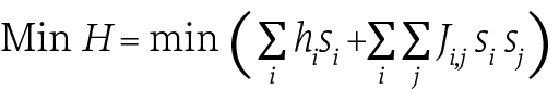
As can be seen, this shape is very similar to the formulation of the QUBO in equation: by substituting the magnetic dipole moments –1 and 1 with 0 (asset is not in portfolio), or 1 (asset is in portfolio) we get the relation that the minimum energy value of the Ising problem corresponds to the optimal portfolio of the Markowitz model.
Solving QUBO’s with the Variational Quantum Eigensolver algorithm
After realizing that it is possible to “build” an analogue to the Markowitz problem using atoms, a logical question is: why don’t we do this, and let nature choose our best portfolio? Unfortunately, this is not really feasible: the best portfolio corresponds to the minimum value of the Hamiltonian, but how can we be sure that the equilibrium state that we find, corresponds to this minimum? When we want to build this model of atoms, there are simply too many initial states for the model to try, as this number grows exponentially with the number of atoms: x atoms can assume 2x individual states. For example, a portfolio containing x = 16 assets has over 65,000 different possible combinations, and considering 20 assets results in over a million combinations.
Instead of trying all possible starting states of the Ising model to find the minimum value of the Hamiltonian, hybrid quantum-classic algorithms have been developed, which use minimal quantum resources in conjunction with classic optimization algorithms. One of these algorithms is the Variational Quantum Eigensolver (VQE) ([Qisk21]). So, what do “variational” and “eigen” mean, in this context?
Let’s look at the Hamiltonian of the Ising model again. Simply put, the Hamiltonian is a mathematical function that operates on a physical space, in this case, the dipole moments of the atoms. These kinds of functions are referred to as operators in quantum physics. The physical space in which operators act, is called a state, and in papers usually called |ψ>. One of the fundamental laws of quantum physics relates the Hamiltonian of a system to a system’s energy: H|ψ> = E|ψ>. This famous equation is known as Schrödinger’s equation, and is how quantum physics comes into play in computing! Here, H denotes the Hamiltonian operator, working on state |ψ>, with energy E. States |ψ> that adhere to the above equation are called Eigenstates of a system, with corresponding Eigenvalues E. Interesting to note is that Eigen comes from the German word for own , as these are states and values that are governed by their own operator, but since Germans use capitals for both nouns and names, it was wrongly interpreted as a name and simply copied to English instead of translated.
Schrödinger’s equation is what is solved by the quantum part of the VQE quantum-classic hybrid solver. The quantum operator H is created by stringing several pieces of quantum hardware together. How this can be done will be explained in the next paragraph. By putting in a state |ψ>, the corresponding energy E is found. Going back to the portfolio problem, we mentioned that we want to minimize the Ising Hamiltonian in order to find the best portfolio. This means that we have to find the particular eigenstate |ψ> that corresponds to this minimum energy. But how do we choose this state? As mentioned, the number of states can be enormous for an Ising model, they cannot all be tested. This is where the classic computer comes into play. Instead of trying an infinite set of arbitrary states |ψ>, a classic optimization algorithm can find relations between parameters of |ψ> and the corresponding energy, and limit the search space of the quantum algorithm. Eventually, after sufficient iterations, the parameters of |ψ> are found which minimize the Hamiltonian, and find the optimal portfolio.
Programming a VQE: setting up a quantum circuit
Obviously, the goal of getting quantum-ready is not to hire engineers to build custom hardware to “string together several pieces of quantum hardware”. Instead, large parties such as IBM, Microsoft, and Google provide cloud hardware which allow the user to construct quantum circuits, the quantum equivalent of classical electrical circuits, on general-purpose quantum hardware. A quantum circuit starts with an initial configuration of a number of qubits, which represent the state 
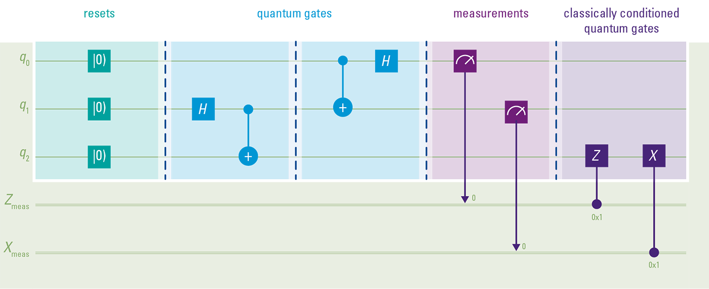
Figure 2. Illustration of a quantum circuit using IBM’s Qiskit library. The above circuit can be defined in various programming languages through the APIs provided in IBM’s Qiskit library, or via a graphical user interface. Upon execution, the circuit can be executed on a simulated quantum computer, or on quantum gates provided by IBM. [Click on the image for a larger image]
Quantum circuits, such as shown in Figure 2, can be programmed in various computer languages, or even with a graphical user interface. Once the user has designed a circuit, jobs are executed on general purpose quantum computers, which prepare the desired initial state, quantum gates, and measurement steps. The analysis can also be carried out on simulated quantum computers. However, when you’re able to formulate your problem in a standardized form such as a QUBO, you can make use of existing algorithms such as the Variational Quantum Eigensolver, and there is no need to design a custom quantum circuit. Solving your problem with a quantum computer can then be done by data scientists or engineers that have some time to familiarize themselves with the principles and pitfalls of the VQE, just like they would have to do with any new algorithm. Since all quantum computations are done behind the scenes, no strong quantum knowledge is required.
The field of developing completely novel quantum algorithms will most likely be the realm of research institutes and dedicated companies, but getting quantum-ready is within reach for all companies with a mindset of change and a healthy desire to experiment and be at the forefront of technology.
Conclusion
Organizations that use mathematical models and algorithms can start with Quantum Computing when certain organizational conditions are met. These conditions are aimed at putting together a team with the proper expertise, and selecting the right use cases that can serve as quantum-computing pilot projects. Implementing and evaluating pilot projects on both classical and quantum computers will give companies hands-on experience with Quantum Computing, whilst building knowledge and a network with quantum providers and the gathered experience will be pivotal in being fully prepared for the era of Quantum Computing!
References
[Carr21] Carrel-Billiar, M. et al. (2021). Get ready for the quantum impact. Accenture. Retrieved from: https://www.accenture.com/_acnmedia/PDF-144/Accenture-Get-Ready-for-the-Quantum-Impact.pdf
[Dilm22] Dilmegani, C. (2022, February 11). Top 20 quantum computing use cases in 2022. AI Multiple. Retrieved from: https://research.aimultiple.com/quantum-computing-applications/
[Goen21] Goense, K., Bertens, R., & Vincelli, R. (2021). Quantum computing, a myth or reality? Compact 2021/2. Retrieved from: https://www.compact.nl/en/articles/quantum-computing-a-myth-or-reality/
[Mark52] Markowitz, H. (1952). Portfolio Selection. The Journal of Finance, 7(1), 77-91. Retrieved from: https://www.jstor.org/stable/i352923
[Marr21] Marr, B. (2021, August 9). The future of quantum computing. Retrieved from: https://bernardmarr.com/the-future-of-quantum-computing/
[McKi21] McKinsey & Company (2021, December). Quantum computing: An emerging ecosystem and industry use cases. Retrieved from: https://www.mckinsey.com/business-functions/mckinsey-digital/our-insights/quantum-computing-use-cases-are-getting-real-what-you-need-to-know
[Micr22a] Microsoft (2022). Azure Quantum. Retrieved from: https://azure.microsoft.com/en-us/services/quantum/
[Micr22b] Microsoft (2022, May 9). Quantum Development Kit (QDK) full state simulator. Retrieved from: https://docs.microsoft.com/en-us/azure/quantum/user-guide/machines/full-state-simulator
[Lipm21] Lipman, P. (2021, January 4). How Quantum computing will transform cyber security. Forbes. Retrieved from: https://www.forbes.com/sites/forbestechcouncil/2021/01/04/how-quantum-computing-will-transform-cybersecurity/?sh=493b133e7d3f
[Niel18] Nielsen, M.A. & Chuang, I.L. (2018). Quantum Computation and Quantum Information. Cambridge University Press.
[Nikh21] Nikhade, A. (2021, June 3). Grover’s search algorithm | simplified. Towards Data Science. Retrieved from: https://towardsdatascience.com/grovers-search-algorithm-simplified-4d4266bae29e
[Prot21] Protiviti (2021). Quantum Computing: why the board should care. Board Perspectives: Risk Oversight [News letter], Issue 139. Retrieved from: https://www.protiviti.com/sites/default/files/newsletter-bpro-issue139-quantum-computing-protiviti.pdf
[QCR21] Quantum Computing Report (2021, November 16). IBM’s Seven Announcements at the IBM Quantum Summit. Retrieved from: https://quantumcomputingreport.com/ibms-seven-announcements-at-the-ibm-quantum-summit/
[Qisk21] Qiskit (2021). VQE. Retrieved from: https://qiskit.org/documentation/stubs/qiskit.algorithms.VQE.html
[Yndu19] Yndurain, E., Woerner, S., & Egger, D. (2019). Exploring quantum computing use cases for financial services. IBM. Retrieved from: https://www.ibm.com/downloads/cas/2YPRZPB3